Intro to R and RStudio
Julie Lowndes
August 17, 2017
Background
You are all here today to learn how to code. Coding made me a better scientist because I was able to think more clearly about analyses, and become more efficient in doing so. Data scientists are creating tools that make coding more intuitive for new coders like us, and there is a wealth of awesome instruction and resources available to learn more and get help.
Here is an analogy to start us off. If you were a pilot, R is an an airplane. You can use R to go places! With practice you’ll gain skills and confidence; you can fly further distances and get through tricky situations. You will become an awesome pilot and can fly your plane anywhere.
And if R were an airplane, RStudio is the airport. RStudio provides support! Runways, communication and other services, and just makes your overall life easier. So although you can fly your plane without an airport and we could learn R without RStudio, that’s not what we’re going to do.
We are learning R together with RStudio and its many supporting features.
Something else to start us off is to mention that you are learning a new language here. It’s an ongoing process, it takes time, you’ll make mistakes, it can be frustrating, but it will be overwhelmingly awesome in the long run. We all speak at least one language; it’s a similar process, really. And no matter how fluent you are, you’ll always be learning, you’ll be trying things in new contexts, etc, just like everybody else. And just like any form of communication, there will be miscommunications but hands down we are all better off because of it.
While language is a familiar concept, programming languages are in a different context from spoken languages, but you will get to know this context with time. For example: you have a concept that there is a first meal of the day, and there is a name for that: in English it’s “breakfast”. So if you’re learning Spanish, you could expect there is a word for this concept of a first meal. (And you’d be right: ‘desayuno’). We will get you to expect that programming languages also have words (called functions in R) for concepts as well. You’ll soon expect that there is a way to order values numerically. Or alphabetically. Or search for patterns in text. Or calculate the median. Or reorganize columns to rows. Or subset exactly what you want. We will get you increase your expectations and learn to ask and find what you’re looking for.
OK, let’s get going.
This lesson is a combination of excellent lessons by others (thank you Jenny Bryan and Data Carpentry!) that I have combined and modified for our workshop today. I definitely recommend reading through the original lessons and using them as reference:
R at console, RStudio goodies
Launch RStudio/R.
Notice the default panes:
- Console (entire left)
- Environment/History (tabbed in upper right)
- Files/Plots/Packages/Help (tabbed in lower right)
FYI: you can change the default location of the panes, among many other things: Customizing RStudio.
There are other great features we don’t really have time for today as we walk through the IDE together. (IDE stands for integrated development environment.) Check out the webinar and RStudio IDE cheatsheet for more. (And this is my blog post about RStudio Awesomeness).
Go into the Console, where we interact with the live R process.
Make an assignment and then inspect the object you just created.
x <- 3 * 4
x
## [1] 12In my head I hear, e.g., “x gets 12”.
All R statements where you create objects – “assignments” – have this form: objectName <- value.
I’ll write it in the command line with a hashtag #, which is the way R comments so it won’t be evaluated.
# objectName <- value

## this is also how you write notes in your code to explain what you are doing.
Object names cannot start with a digit and cannot contain certain other characters such as a comma or a space. You will be wise to adopt a convention for demarcating words in names.
# i_use_snake_case
# other.people.use.periods
# evenOthersUseCamelCase
Make an assignment
this_is_a_really_long_name <- 2.5To inspect this variable, instead of typing it, we can press the up arrow key and call your command history, with the most recent commands first. Let’s do that, and then delete the assignment:
this_is_a_really_long_name## [1] 2.5Another way to inspect this variable is to begin typing this_…and RStudio will automagically have suggested completions for you that you can select by hitting the tab key, then press return.
And another way to inspect this is by looking at the Environment pane in RStudio.
this_is_a_really_long_name## [1] 2.5One more:
science_rocks <- 2Let’s try to inspect:
sciencerocks## Error in eval(expr, envir, enclos): object 'sciencerocks' not foundImplicit contract with the computer / scripting language: Computer will do tedious computation for you. In return, you will be completely precise in your instructions. Typos matter. Case matters. You’ll need to pay attention to how you type.
Remember that this is a language, not unsimilar to English! There are times you aren’t understood – it’s going to happen. There are different ways this can happen. Sometimes you’ll get an error. This is like someone saying ‘What?’ or ‘Pardon’? Error messages can also be more useful, like when they say ‘I didn’t understand this specific part of what you said, I was expecting something else’. That is a great type of error message. Error messages are your friend. Google them (copy-and-paste!) to figure out what they mean.
And also know that there are errors that can creep in more subtly, when you are giving information that is understood, but not in the way you meant. Like if I’m telling a story about tables and you’re picturing where you eat breakfast and I’m talking about data. This can leave me thinking I’ve gotten something across that the listener (or R) interpreted very differently. And as I continue telling my story you get more and more confused… So write clean code and check your work as you go to minimize these circumstances!
A moment about logical operators and expressions. We can ask questions about the objects we just made.
==means ‘is equal to’!=means ‘is not equal to’<means ` is less than’>means ` is greater than’<=means ` is less than or equal to’>=means ` is greater than or equal to’
science_rocks == 2## [1] TRUEscience_rocks <= 30## [1] TRUEscience_rocks != 5## [1] TRUEShortcuts You will make lots of assignments and the operator
<-is a pain to type. Don’t be lazy and use=, although it would work, because it will just sow confusion later. Instead, utilize RStudio’s keyboard shortcut: Alt + - (the minus sign). Notice that RStudio automagically surrounds<-with spaces, which demonstrates a useful code formatting practice. Code is miserable to read on a good day. Give your eyes a break and use spaces. RStudio offers many handy keyboard shortcuts. Also, Alt+Shift+K brings up a keyboard shortcut reference card.
My most common shortcuts include command-Z (undo), and combinations of arrow keys in combination with shift/option/command (moving quickly up, down, sideways, with or without highlighting.
When assigning a value to an object, R does not print anything. You can force R to print the value by using parentheses or by typing the object name:
weight_kg <- 55    # doesn't print anything
(weight_kg <- 55)  # but putting parenthesis around the call prints the value of `weight_kg`
## [1] 55weight_kg # and so does typing the name of the object## [1] 55Now that R has weight_kg in memory, we can do arithmetic with it. For instance, we may want to convert this weight into pounds (weight in pounds is 2.2 times the weight in kg):
2.2 * weight_kg## [1] 121We can also change a variable’s value by assigning it a new one:
weight_kg <- 57.5
2.2 * weight_kg
## [1] 126.5This means that assigning a value to one variable does not change the values of other variables. For example, let’s store the animal’s weight in pounds in a new variable, weight_lb:
weight_lb <- 2.2 * weight_kgand then change weight_kg to 100.
weight_kg <- 100What do you think is the current content of the object weight_lb? 126.5 or 220?
R functions, help pages
R has a mind-blowing collection of built-in functions that are accessed like so
# function_name(argument1 = my_first_argument, argument2 = my_second_argument...)Let’s try using seq() which makes regular sequences of numbers and, while we’re at it, demo more helpful features of RStudio.
Type se and hit TAB. A pop up shows you possible completions. Specify seq() by typing more to disambiguate or using the up/down arrows to select. Notice the floating tool-tip-type help that pops up, reminding you of a function’s arguments. If you want even more help, press F1 as directed to get the full documentation in the help tab of the lower right pane.
Type the arguments 1, 10 and hit return.
seq(1, 10)## [1] 1 2 3 4 5 6 7 8 9 10We could probably infer that the seq() function makes a sequence, but let’s learn for sure. Type (and you can autocomplete) and let’s explore the help page:
?seq
help(seq) # same as ?seq
seq(from = 1, to = 10) # same as seq(1, 10); R assumes by position
## [1] 1 2 3 4 5 6 7 8 9 10seq(from = 1, to = 10, by = 2)## [1] 1 3 5 7 9The above also demonstrates something about how R resolves function arguments. You can always specify in name = value form. But if you do not, R attempts to resolve by position. So above, it is assumed that we want a sequence from = 1 that goes to = 10. Since we didn’t specify step size, the default value of by in the function definition is used, which ends up being 1 in this case. For functions I call often, I might use this resolve by position for the first argument or maybe the first two. After that, I always use name = value.
The help page tells the name of the package in the top left, and broken down into sections:
- Description: An extended description of what the function does.
- Usage: The arguments of the function and their default values.
- Arguments: An explanation of the data each argument is expecting.
- Details: Any important details to be aware of.
- Value: The data the function returns.
- See Also: Any related functions you might find useful.
- Examples: Some examples for how to use the function.
The examples can be copy-pasted into the console for you to understand what’s going on. Remember we were talking about expecting there to be a function for something you want to do? Let’s try it. min(), max(), log()…
Exercise: Talk to your neighbor(s) and look up the help file for a function you know. Try the examples, see if you learn anything new. (need ideas?
?getwd(),?plot(),?mean(),?log()).
Help for when you only sort of remember the function name: double-questionmark:
??install Not all functions have (or require) arguments:
date()## [1] "Thu Aug 17 12:14:33 2017"Now look at your workspace – in the upper right pane. The workspace is where user-defined objects accumulate. You can also get a listing of these objects with commands:
objects()## [1] "science_rocks" "this_is_a_really_long_name"
## [3] "weight_kg" "weight_lb"
## [5] "x"ls()## [1] "science_rocks" "this_is_a_really_long_name"
## [3] "weight_kg" "weight_lb"
## [5] "x"If you want to remove the object named weight_kg, you can do this:
rm(weight_kg)To remove everything:
rm(list = ls())or click the broom in RStudio’s Environment pane.
Exercise: Clear your workspace, then create a few new variables. Create a variable that is the mean of a sequence of 1-20. What’s a good name for your variable? Does it matter what your ‘by’ argument is? Why?
Working directories, RStudio projects, scripts
So we will talk about scripts in a moment, but first let’s talk about where they should live.
We’re not going to cover workspaces today, but this is another alternative to scripts. You can learn about it in this RStudio article: Working Directories and Workspaces.
Working directory
Any process running on your computer has a notion of its “working directory”. In R, this is where R will look, by default, for files you ask it to load. It is also where, by default, any files you write to disk will go. You have a sense of this because whenever you go to save a Word doc or download, it asks where. You often have to navigate to put it exactly where you want it. There are a few ways to check your working directory in RStudio.
You can explicitly check your working directory with:
getwd()It is also displayed at the top of the RStudio console.
As a beginning R user, it’s OK let your home directory or any other weird directory on your computer be R’s working directory. Very soon, I urge you to evolve to the next level, where you organize your analytical projects into directories and, when working on Project A, set R’s working directory to Project A’s directory.
You can set R’s working directory at the command line like so. You could also do this in a script.
setwd("~/myCoolProject")But there’s a better way. A way that also puts you on the path to managing your R work like an expert.
RStudio projects
Keeping all the files associated with a project organized together – input data, R scripts, analytical results, figures – is such a wise and common practice that RStudio has built-in support for this via its projects. More here: Using Projects.
Let’s make one to use for the rest of today.
Do this: File > New Project … New Directory > Empty Project. The directory name you choose here will be the project name. Call it whatever you want (or follow me for convenience).
I created a directory and, therefore RStudio project, called data-carpentry in a folder called tmp in my home directory, FYI. What do you notice about your RStudio pane? Look in the right corner–‘data-carpentry’.
Now check that the “home” directory for your project is the working directory of our current R process:
getwd()
# "/Users/julialowndes/tmp/data-carpentry"
About paths: The above is the absolute path: it starts at the /Users root and is specific to my computer (julialowndes) and where I saved it. So if I did an analysis with this filepath, it wouldn’t work on your computer before you altered the filepath.
But with an RStudio project, your paths within this project can be relative, which means they start in the data-carpentry folder, wherever it is. So we can just use filepaths within our project from a relative place, and it can work on your computer or mine, without worrying about the absolute paths. (Analogy: I can give you directions from this building to the pub, since we’re all here in this shared space already. I can’t give you all directions from your home to this building and then the pub, because you all live in different places. But I can give directions relative to this building).
Create an R script
It’s been great to play around in the console, but we are really here to focus on reproducible analyses, and that means saving our work in a script that can be rerun. Create a new R script by going to File > New File > R Script or going to the little plus at the top left of the RStudio console. Put a comment at the top of this script for now:
## 2017-08-17-my-script.r
## Julie Lowndes lowndes@nceas.ucsb.edu
Click on the floppy disk to save. Give it a name ending in .R or .r, and use no spaces in the name. I named mine 2017-08-17-my-script.r and note that, by default, it will go in the directory associated with your project. It is traditional to save R scripts with a .R or .r suffix. (check out Jenny Bryan’s rules for naming filesnames here)
Create a data folder
Let’s also create a folder in our Project called ‘data’ (all lowercase). You can do this in your Finder/Windows Explorer as you would normally, or you can do it from RStudio, using the Files tab in the bottom right pane.
Download and save our data
We will use the download.file() function to download data from figshare online. Let’s look up ?download.file() in the help first.
Let’s run this. Unlike when we typed in the console, hitting ‘enter’/‘return’ won’t execute the command; we’ve essentially just written it in a text file. So to execute it, we’ll have to press the ‘Run’ button in the top right of the editor pane, or a shortcut is command-enter.
download.file("https://ndownloader.figshare.com/files/2292169",
              "data/portal_data_joined.csv")
A few things to note with the above: the function call is written across 2 lines: R is OK with extra white space, and will even indent so it’s easier to read.
Once you run this, you should see the file appear in the data folder.
Explore the data
Let’s read the data into R and save it to a variable called surveys. Type this into your script.
## read in the data
surveys <- read.csv("data/portal_data_joined.csv")
Now, we are going to start exploring data. Click on ‘surveys’ in the environment pane.
Luckily, this data frame is tidy: (from the RStudio data wrangling cheatsheet):
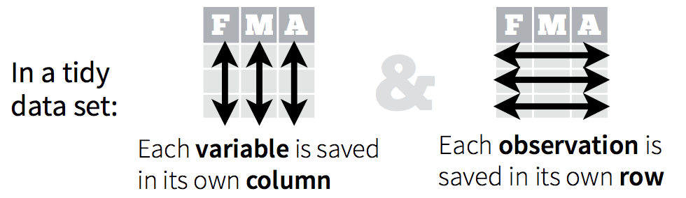
We are studying the species and weight of animals caught in plots in our study area. The dataset is stored as a comma separated value (CSV) file. Each row holds information for a single animal, and the columns represent:
| Column | Description |
|---|---|
| record_id | Unique id for the observation |
| month | month of observation |
| day | day of observation |
| year | year of observation |
| plot_id | ID of a particular plot |
| species_id | 2-letter code |
| sex | sex of animal (“M”, “F”) |
| hindfoot_length | length of the hindfoot in mm |
| weight | weight of the animal in grams |
| genus | genus of animal |
| species | species of animal |
| taxa | e.g. Rodent, Reptile, Bird, Rabbit |
| plot_type | type of plot |
Let’s try this without using the mouse, we can type commands in our script too. Type surveys and execute this line by pressing ‘Run’ or command-return.
surveys # this is super long! Let's inspect in different waysLet’s use head and tail:
head(surveys) # shows first 6
tail(surveys, 10) # guess what this does!
str() will provide a sensible description of almost anything: when in doubt, just str() some of the recently created objects to get some ideas about what to do next.
str(surveys) # ?str - displays the structure of an objectsurveys is a data.frame. We aren’t going to get into the other types of data receptacles today (‘arrays’, ‘matrices’), because working with data.frames is what you should primarily use. Why?
- data.frames package related variables neatly together, great for analysis
- most functions, including the latest and greatest packages actually require that your data be in a data.frame
- data.frames can hold variables of different flavors such as
- character data (genus or sex; “Factors”)
- quantitative data (record_id, year; “Integers (int)” or “Numeric (num)”)
- categorical information (male vs. female)
Inspecting data.frame Objects
We already saw how the functions head() and str() can be useful to check the content and the structure of a data frame. Here is a non-exhaustive list of functions to get a sense of the content/structure of the data. Let’s try them out!
Explore content:
## explore content
head(surveys) # first 6 rows
tail(surveys) # last 6 rows
tail(surveys, 10) # last 10 rows
Summaries:
## summaries
str(surveys) # structure of the object and information about the class, length and content of  each column
summary(surveys) # summary statistics for each column
Explore size:
## size
dim(surveys) # number of rows and the number of columns (the dimensions)
nrow(surveys) # number of rows
ncol(surveys) # number of columns
Explore names:
## names
names(surveys) # column names
Note: most of these functions are “generic”, they can be used on other types of objects besides data.frame.
Look at the variables inside a data.frame
To specify a single variable from a data.frame, use the dollar sign $. The $ operator is a way to extract of replace parts of an object–check out the help menu for $. It’s a common operator you’ll see in R.
surveys$weight # very long! hard to make sense of...
head(surveys$weight) # can do the same tests we tried before
str(surveys$weight) # it is a single numeric vector
summary(surveys$weight) # same information, just formatted slightly differently
We’ll spend tomorrow talking more about visualization, but it’s so important for smell-testing dataset that we will make a few figures anyway. Here we use only base R graphics, which are very basic.
## plot surveys
plot(surveys$year, surveys$weight) # ?plot
plot(surveys$hindfoot_length, surveys$weight)
There is a lot of data here, but these plots can help us think about the data and what we may want to explore further. For example, could those differences hindfoot_length vs weight be explained by sex?
Let’s explore another numeric variable: life expectancy.
## explore numeric variable
summary(surveys$month)
hist(surveys$month)
Let’s explore a categorical variable (stored as a factor in R): continent.
## explore factor variable
summary(surveys$taxa)
levels(surveys$taxa)
nlevels(surveys$taxa)
hist(surveys$taxa) # whaaaa!?
This error is because of what factors are ‘under the hood’: R is really storing integer codes 1, 2, 3 here, but represent them as text to us. Factors can be problematic to us because of this, but you can learn to navigate with them. There are resources to learn how to properly care and feed for factors.
One thing you’ll learn is how to visualize factors with which functions/packages.
class(surveys$taxa) # ?class returns the class type of the object
table(surveys$taxa) # ?table builds a table based on factor levels
class(table(surveys$taxa)) # this has morphed the factor...
barplot(table(surveys$taxa)) # so we can plot!
I don’t want us to get too bogged down with what’s going on with table() and plotting factors, but I want to expose you to these situations because you will encounter them. Googling the error messages you get, and knowing how to look for good responses is a critical skill. (I tend to look for responses from stackoverflow.com that are recent and have green checks, and ignore snarky comments).
Subsetting data
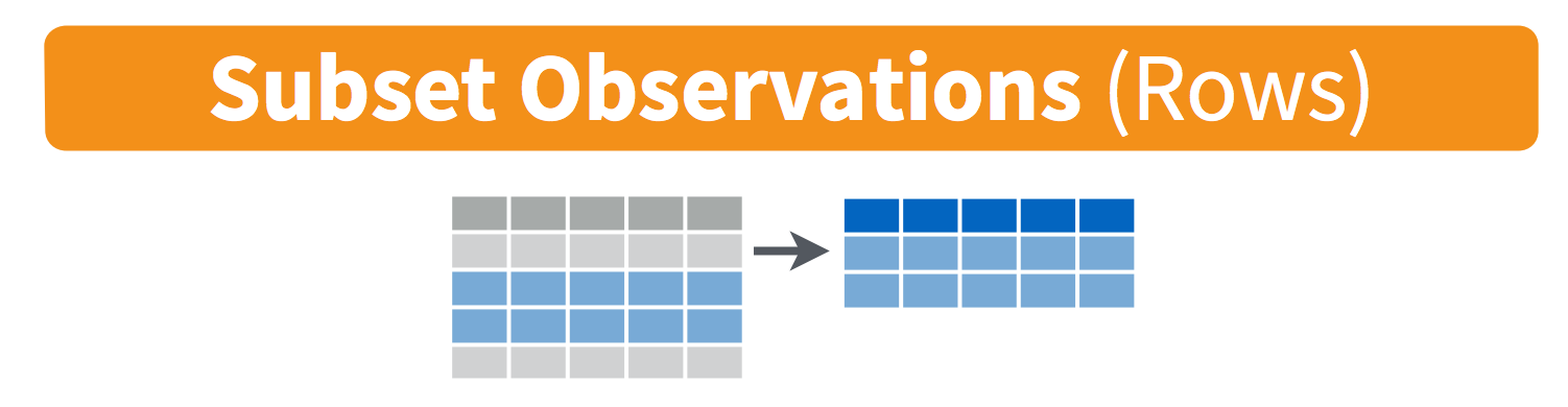
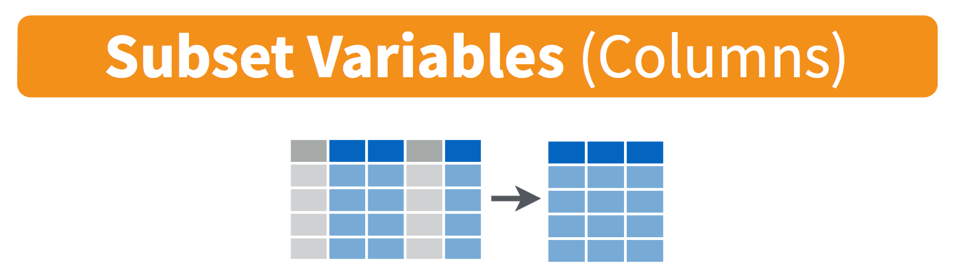
You will want to isolate bits of your data; maybe you want to just look at a single species or a few years. R calls this subsetting. There are several ways to do this. We’ll go through a few options in base R so that you’re familiar with them, and know how to read them. But then we’ll move on to a new, better, intuitive, and game changing way with the dplyr package tomorrow.
Visually, we are doing this (thanks RStudio for your cheatsheet): (these images are from RStudio cheatsheets for dplyr and tidyr, which we will talk about all tomorrow).
Selecting across rows is called filtering:
Selecting across rows is called selecting:
subsetting with base [rows, columns] notatation
Remember your logical expressions from this morning? We’ll use == here.
This notation is something you’ll see a lot in base R. the brackets [ ] allow you to extract parts of an object. Within the brackets, the comma separates rows from columns.
## subset numeric data
surveys[surveys$month >2, ] # don't forget this comma!

## subset factors
surveys[surveys$taxa == "Reptile", ] # don't forget this comma!
So our notation is saying ‘select these rows, and all columns’.
We could also select which columns to keep using the c() function:
surveys[surveys$taxa == "Reptile", c("record_id", "year", "weight", "taxa")] # ?c: combines values into a vector or listContrast the above command with this one accomplishing the same thing:
surveys[c(2010,4933,6933,12710,12718,14015,14016), ] # No idea what we are inspecting. Don't do this. And, I introduced a typo!

surveys[c(2010,4933,6993,12710,12718,14015,14016), c(1, 4, 9, 12)] # Ditto.
Yes, these both return the same result. But the second command is horrible for these reasons:
- It contains Magic Numbers. The reason for keeping rows 1621 to 1632 will be non-obvious to someone else and that includes you in a couple of weeks.
- It is fragile. If the rows of
surveysare reordered or if some observations are eliminated, these rows may no longer correspond to the Reptile data.
In contrast, the first command, is somewhat self-documenting; one does not need to be an R expert to take a pretty good guess at what’s happening. It’s also more robust. It will still produce the correct result even if surveys has undergone some reasonable set of transformations (what if it were in in reverse alphabetical order?)
Clean up our R script
Here is what mine looks like:
## 2017-08-17-my-script.r
## Julie Lowndes lowndes@nceas.ucsb.edu

## read in the data
download.file("https://ndownloader.figshare.com/files/2292169",
              "data/portal_data_joined.csv")
surveys <- read.csv("data/portal_data_joined.csv")

## explore content
head(surveys) # first 6 rows
tail(surveys) # last 6 rows
tail(surveys, 10) # last 10 rows

## summaries
str(surveys) # structure of the object and information about the class, length and content of  each column
summary(surveys) # summary statistics for each column

## size
dim(surveys) # number of rows and the number of columns (the dimensions)
nrow(surveys) # number of rows
ncol(surveys) # number of columns

## names
names(surveys) # column names

## explore numeric variables
surveys$weight # very long! hard to make sense of...
head(surveys$weight) # can do the same tests we tried before
str(surveys$weight) # it is a single numeric vector
summary(surveys$weight) # same information, just formatted slightly differently

## quick plots of numeric variables
plot(surveys$year, surveys$weight) # ?plot
plot(surveys$hindfoot_length, surveys$weight)

## explore factor variable
class(surveys$taxa)
summary(surveys$taxa)
levels(surveys$taxa)
nlevels(surveys$taxa)
barplot(table(surveys$taxa))

## subset numeric variables
surveys[surveys$month >2, ] # don't forget this comma!

## subset factors
surveys[surveys$taxa == "Reptile", ] # don't forget this comma!

## subset variables and only retain certain columns
surveys[surveys$taxa == "Reptile", c("record_id", "year", "weight", "taxa")] # ?c: combines values into a vector or list

## never subset this way! Magic numbers are bad!
surveys[c(2010,4933,6993,12710,12718,14015,14016), c(1, 4, 9, 12)] # What does this even mean?
Remember…
This workflow will serve you well in the future:
- Create an RStudio project for an analytical project
- Keep inputs there (although we didn’t save data locally, we put it directly into the R workspace for now)
- Keep scripts there; edit them, run them in bits or as a whole from there
- Keep outputs there (we’ll do that tomorrow) Avoid using the mouse for pieces of your analytical workflow, such as loading a dataset or saving a figure. This is terribly important for reproducility and for making it possible to retrospectively determine how a numerical table or PDF was actually produced (searching on local disk on filename, among
.Rfiles, will lead to the relevant script).